Traps of Custom Formatting

Numbers can coexist in Excel cells with text strings. What may surprise you is that the contents of such cells can be treated and used as numbers. It means that they can be used as ordinary numbers in mathematical calculations, functions and formulas. This happens when you apply some kinds of custom formatting for cells.

Here is such example of cell formatting and some confusing results of using it in formulas involving text strings.

I've used the following custom format for cells in column A:

Conditional Formatting in Excel: All you need to know

This is about visual identification and/or formatting (differentiation) of our data sets based on our questions (conditions), in order to: 

• mark/reveal some data of interest, present them
  
• take some action (e.g. find errors, correct, sort, delete, evaluate), or
• find out some trends and patterns, compare.

Here is the Conditional Formatting main menu (on the left) + More Rules dialog:

How to REPLACE any substrings or COUNT them in a string

Let's say we are dealing with the following string entered in cell A1:

"Examples of replacing or counting any string elements in a cell"

To replace e.g. the 3rd letter 'a' with 'A' in the string, we would use this formula:

=SUBSTITUTE($A$1,"a","A",3)

To count e.g. the number of SPACES in the string, the following formula can be used:

=LEN($A$1) -LEN(SUBSTITUTE($A$1," ",""))        (result = 10)

To count the number of substrings, such as e.g. "e", "in", "le" or "count" in the string, the following formulas can be used:

• =(LEN($A$1) -LEN(SUBSTITUTE($A$1,"e","")))/LEN("e")    (result = 6)
• =(LEN($A$1) -LEN(SUBSTITUTE($A$1,"in","")))/LEN("in")    (result = 4)
• =(LEN($A$1) -LEN(SUBSTITUTE($A$1,"le","")))/LEN("le")    (result = 2)
• =(LEN($A$1) -LEN(SUBSTITUTE($A$1,"count","")))/LEN("count")     (result = 1)

 

Template for Basic Data Summary/Analysis

If you have collected and organized some data in table(s) or list(s), the first thing you might need could be to get quick general analysis/evaluation of that data - before going any further with some math, statistical or graphic analysis.

The following example provides easy solution, kind of a template, for that preliminary summary and basic analysis.

Here's just illustrative table of random data. Let's say you want to know "everything" about this set of values.

Extract Formulas to External File

If your workbook/worksheet is full of Excel formulas it may be worth to keep track of them in one place, in a compact listing, in a separate text file.

Here is a simple short macro that serves the purpose:

Sub ListFormulas()
Dim rng As Range
'Extracts all formulas from a worksheet to a text file (Notepad/Wordpad)
Open "C:\Users\Adam\Desktop\XFormulas.txt" For Output As #1
For Each rng In Sheets("Formulas").UsedRange.Cells

If rng.Formula <> "" And Left(rng.Formula, 1) = "=" Then
           Print #1, rng.Address; Tab; rng.Formula
End If

Next
Close #1
End Sub

Data entry tips: Formulas and Dates

You might learn from some sources that when you enter a formula into a cell in Excel, you have to start your entry always with the equal sign. This is not true. You can, but DON'T NEED to start with the '=' sign.

Each formula can be started also with either '+', or '-' (if you mean negative number/expression) signs. When you press the ENTER key, Excel will voluntarily add the equal sign for you.

Here are couple of examples to illustrate what happens:

 

How to create MUTUALLY DEPENDENT CELLS

Mutual dependence of Excel cells means that some two cells in your workbook refer to each other. If the value of one of the two dependent cells changes it causes change of value in the other cell dependent on it. This normally leads to a problem called "circular reference". However, it is possible to set up mutually dependent cells by following steps shown in my example below.

TIPS for CLICKS: Working with Functions and Formulas

Excel FUNCTIONS = Predefined formulas used for specific values in a specific order. They operate usually on data entered in range of cells and increase the Excel users productivity. Total number of the functions available in Excel is close to 700.

Some of the most important of them (most frequently used) are: SUM, IF, MIN, MAX, AND, OR, AVERAGE, COUNT, DAYS, VLOOKUP, DATE, ... etc. Examples of functions working with text: UPPER, LOWER, PROPER,... etc.

Excel FORMULAS = Expressions operating on values in a range of cells and operators. Can utilize several Excel functions and work with both numeric and textual data. ARRAY formulas are a special type of formulas, and can be very complex.

Here is the list and description of some of the most useful shortcuts used in conjunction with Functions and Formulas. I hope you'll find them helpful.

Font color change within cell formula

Formulas in Excel usually don't care about the font color in displaying their results in a cell. However, you may need sometimes to distinguish between some results of your calculations by using specific font colors.

It is possible to assign a specific font color to a cell value, without any conditional formatting.

E.g., let's say, you want to compare two numbers (located in cells A1 and B1) and assign font color to the result of the formula like this one: =IF(A1>B1,22,33).  Depending on the outcome of comparison, if A1>B1 then you want to display 22 in green color; otherwise you want to display 33 in red.

To do that with a formula, you need to amend the formula with this kind of UDF (user defined function): 

 Function CFcolor(num1 As Double, num2 As Double) As Boolean
    If num1 <= num2 Then
        Application.Caller.Font.ColorIndex = 3       'red
    Else
        Application.Caller.Font.ColorIndex = 10     'green
    End If
End Function 

so that your formula looks like this:  =IF(A1>B1,22,33)+CFcolor(A1,B1) .

Obviously, to make use of the function, you have to copy and paste it first into a Module of your VBAProject (your workbook) or of your Personal workbook.

The function can be quite easily modified for use with other Excel formulas and colors.

 

How to create a 'slide show' using a single formula and a chart

If you want to make use of some math formulas for practical applications or just to show off your Excel creativity, you can utilize kind of slide show: = refreshable charts based on your brilliant formula.

Follow these steps:

• Open a new workbook. Enter any two numbers into your worksheet (Sheet1), e.g. 1 in cell A2 and 2 in B2.
• Start with creating a simple XY scatter chart based on your entries. This chart is named as "Chart 1".
• Delete the two numbers you've just entered. You don't need them.
• Expand the width of column A to e.g. 200, move there the chart and resize it to the size of your choice.
• In cell D1, type the formula you want to chart, in the format using explicitly normal math signs and functions, e.g. x^2+5*sqrt(x)-3 .
• Enter the low and high limits (of your choice) for the Left value and the Right value of x axis, then also the Low and High limits for the number of Points you want to be plotted, as shown in the example below (cells D3:E5).
• In cells F3:F5, enter RANDBETWEEN formulas as shown in the example, cells F3:F5.

CHARTS: How to plot nice chart for any formula / equation

Would you like to create impressive charts effortlessly, based just on a single formula? Would you like your charts look similar to these examples? If so, follow the directions below.

 

 

One of interesting features related to charting in Excel allows you to plot charts based not on actual data ranges/tables but based on formulas.

Here are the basic steps to follow if you'd like to create such nice charts quickly. If you create just one of them, you can save the file as a template for future use.

The first thing to do is to enter/arrange all necessary information you'll need for your chart elements. So, enter the following in your worksheet:

Cell	Text entry	Cell	Data entry
A1	“Formula to plot”	B1	Enter/paste your formula to be plotted
A2	“xLeft”	B2	Enter number for starting point of X axis
A3	“xRight”	B3	Enter number for ending point of X axis
A4	“Number of points”	B4	Enter number of points to be plotted
A5	“Chart title”	B5	Enter “Plott for: “Sheet1!$B$1
A7	“List of formulas”
A8	Enter your first formula, e.g. x^3+20^2-100*x
A9	and 2nd one, e.g. (sqrt(cos(x))*cos(500*x)+sqrt(abs(x))-0.4)*(4-x*x)
A10	Etc….

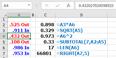
When you enter all required information your worksheet may look similar to this one:

 

Remember that you have to follow the format of the formulas exactly as shown here in the examples. No free spaces are allowed within the equation; they would create error message. Remember also that you can change the plot view by changing coordinates and number of points plotted (entries in cells B2:B4).

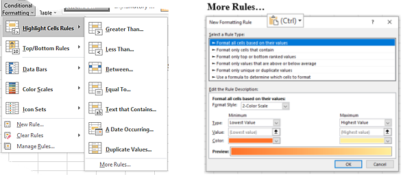
The second thing to do is to define some Names. On Formulas tab, in "Define Names group, click "Define Name" and define the following Names, one by one:

Name	Refers To:
Formula	=Sheet1!$B$1
xLeft	=Sheet1!$B$2
xRight	=Sheet1!$B$3
xNoOfPoints	=Sheet1!$B$4
xRng	=xRight-xLeft
x	=xLeft+xRng/(xNoOfPoints-1)*(ROW(OFFSET(Sheet1!$A$1,0,0,xNoOfPoints,1))-1)
y	=EVALUATE(Sheet1!$B$1 & ”+0*x”

Now, select any area in your worksheet and, in your the Menu Bar select Insert>Charts>Insert Scatter(X,Y)... Select one of Scatter charts. Place the chart conveniently in your worksheet and right-click on the chart area. In Edit Series window, click on Edit button and in Edit Series window enter:

• under Series name: select range B5 in the worksheet,
• under Series X values: enter "=Shee1!x"
• under Series Y values: enter "=Sheet1!y"

Now you can format your data points in the chart. Right-click in chart area and select Change Chart Type. Select All Charts and click on 3-D Bubble icon. Click OK.

Next, right-click on data points (markers) and select Format Data Series... . Click on Series Options icon () , set the Scale bubble size to e.g. 15 (Area of bubbles), then click on Fill & Line icon (), select Fill>Automatic and mark Vary colors by point.

If you need to edit/add chart title, right-click on the title box and either:

• select Edit Text and edit it, or
• in Formula Bar enter "=" and select cell B5.

Select the chart, click on Chart Elements icon () and select those elements which you want to be displayed in the chart (titles, axes, gridlines, data labels, error bars, legend, trendline). Make any changes you want to those elements.

Select the chart and click on Chart Styles icon () and select your favorite style and color scheme for your chart.

Have you got any interesting chart? If so, please share it with me.