Traps of Custom Formatting

Numbers can coexist in Excel cells with text strings. What may surprise you is that the contents of such cells can be treated and used as numbers. It means that they can be used as ordinary numbers in mathematical calculations, functions and formulas. This happens when you apply some kinds of custom formatting for cells.

Here is such example of cell formatting and some confusing results of using it in formulas involving text strings.

I've used the following custom format for cells in column A:

Picture in Picture in Excel Worksheet

What if you need to highlight/call attention to any fragment of your worksheet, be it a piece of data table or a picture/chart, for a presentation or just for printing a report?

You can do it quite easily in Excel. Let's consider a picture. You may need to overlay an enlarged small fragment of your picture onto the original whole picture. To do that you can use the Windows "Snip & Sketch" utility (the shortcut to invoke it, is: Windows Logo key + SHIFT + S). You can select either rectangular or free-form snip. After getting the snip, format/enlarge it as needed, in a way attracting attention to it, and move it to a desired position. This is an example of the 'picture in picture':

The same can be done also with any chart/graphics.

How to find out if there are hidden data in Excel cells

You probably know how to hide some values in Excel cells. If not, this is how it can be done:

• select Home>Format in the Cells group, and then
• Format Cells...>Number>Custom, and then
  
• create the ; or ;; (single or double semicolon) and/or ;;; (triple semicolon) formats

With ; or ;; format you will be able to hide numeric values, and with ;;; format - all textual and numeric values.

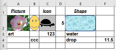
The hiding of values can be enhanced with covering the cells with some graphics (pictures, icons or shapes) as you can see in this simple example:

Cells A2,C2 and E2 in this example are custom-formatted with ;;; so each of them may hold a hidden value. Cell A2 holds number 32.58, cell E2 holds value "TEXT" and cell C2 is left blank (no value). Cell B2 holds number 7 and is not custom-formatted. The range I've selected here is A1:F5. The graphics are used in this example just for masking; they are displayed in the top layer of the cells and may be used to hide even not custom-formatted cell value (like in cell B2).

Now, the question is, how you can determine if there are any hidden values within a selected range of cells. Even if you yourself created the spreadsheet some time ago, you may not remember if there are any hidden cell values and would like to check that.

You can use quite straightforward procedure to do that:

• select the range you want to check
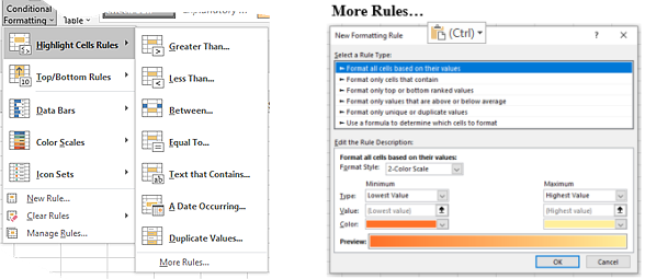
• in the ribbon select Home>Conditional formatting (in Styles group) >Highlight Cells Rules>Text that Contains... 
• under Format cells that contain the text: box enter * only and select highlighting option, e.g. Green Fill... , then click OK.

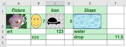
You'll see green-highlighted all cells that contain some values, including the hidden values.

If any of the cells are 'masked' with graphics, you may need to check them individually by temporarily resizing/moving them to see underlying content (if any). This way you'll know that all the green-highlighted cells contain values (doesn't matter if looking like blank or covered with graphics). Cells A2 and E2 have also been highlighted with green. It means there are hidden values entered there. Clicking on green areas show their content in the Formula Bar.

Later on, you can remove the highlighting, if no longer needed. In the meantime, by using some formulas, you can make a number of different checks on the cells in the selected range to confirm existence of cells with hidden values. E.g.:

• =COUNT(A1:F5)      Counts cells with numeric values in the selected range
  
• =COUNTA(A1:F5) or =COUNTIF(A1:F5,"<>") or =SUBTOTAL(103,A1:F5)    Count cells with any value (not empty) in the selected range
  
• =SUM(A1:F5)      Returns the sum of numeric values in the selected range
  
• =ISTEXT(E2)       Returns TRUE if the cell contains text
• =COUNTIF(A1:F5,"")  or  =ROWS(A1:F5)*COLUMNS(A1:F5)-SUBTOTAL(103,A1:F5)     Return count of blank cells in the selected range
• =IF(CELL("format",A2)="H","H","-")     Returns "H" if the selected cell is custom-formatted to hide entered value
  

The last formula can be used to check for hidden values within the whole range/table of data.

 

Conditional Formatting in Excel: All you need to know

This is about visual identification and/or formatting (differentiation) of our data sets based on our questions (conditions), in order to: 

• mark/reveal some data of interest, present them
  
• take some action (e.g. find errors, correct, sort, delete, evaluate), or
• find out some trends and patterns, compare.

Here is the Conditional Formatting main menu (on the left) + More Rules dialog: