Excel Secrets: Dates in Charts

Something strange happens with Excel charts when you create a chart based on data that include column of dates in the selected data range. Here is an example of simple data set I'm using as basis for my charts:

This is my first selected type of chart. Everything looks OK, dates on X axis are displayed correctly:

Now, when I create (or switch to) some different types of my chart, here's what I'm getting:

The X axis presents here completely different dates in different steps from those listed in my table. Why is this happening? Does anybody know? Is this one of Excel tricks?

For now just be aware of this abnormality and examine your charts well before using/publishing them.

 

Excel Interface: Hide or Restore

Normally, Excel application displays user interface (ribbon standard) like this (top and bottom parts):

Workbook Events: Printing - Speach - Alerts

When printing in Excel, one quite frequently makes mistakes. Sometimes the printout does not look as expected and we may waste more paper than necessary. To reduce such outcomes to minimum we can utilize Excel event feature called BeforePrint.

You can use the following workbook event procedure (VBA code) that will - just before printing your worksheet/selection - alert you with speech feature by asking if you are sure that your workbook and the print settings are OK; if not, printing is cancelled.

Private Sub Workbook_BeforePrint(Cancel As Boolean)
 For Each wk In Worksheets  'Make sure that worksheets are recalculated before printing
    wk.Calculate
 Next
 vbOption = MsgBox("Are you sure that all settings are OK and print can be started?", vbYesNo)
 If vbOption = 7 Then   '6=Yes, 7=No
    Cancel = True
    Application.Speech.Speak "Print is cancelled."
'    MsgBox ("Print is cancelled.") 'optional
    Else
        Application.Speech.Speak "Recalculation is completed and now printing takes place."
    End If
End Sub

To implement this procedure, select the Developer tab in the ribbon and select Visual Basic from the menu, then select the View tab>Project Explorer. In VBAProject of your workbook click on ThisWorkbook, then copy the code provided here and paste it into the space located directly under the Workbook field there. Save your workbook as Excel Macro-Enabled Workbook.

Try to print something to see if the event procedure works as intended.

 

Wonders of Excel: FILL HANDLE

As you probably know, Excel Fill Handle is located in the bottom right of any active cell or the bottom right cell of a selected range. It's a quite small black square visible in this snip:

Small it is, but it's very important to know how to utilize it, as it can be really helpful in eliminating lots of manual typing and saving time in working with data entry... and much more than this. It can be used for filling any range of cells with increments of any choice you want to select.

To utilize the Fill Handle, first you need to fill one or more cells with values (numbers or text, incl. dates and other custom lists). Hover your mouse pointer over the small square until it changes to a small black cross, then you have couple of choices: you can left-click, right-click or double-click (in some situations); click and drag the mouse in the direction you want to fill up the range of cells with series or custom lists that follow your pre-defined pattern.

Traps of Custom Formatting

Numbers can coexist in Excel cells with text strings. What may surprise you is that the contents of such cells can be treated and used as numbers. It means that they can be used as ordinary numbers in mathematical calculations, functions and formulas. This happens when you apply some kinds of custom formatting for cells.

Here is such example of cell formatting and some confusing results of using it in formulas involving text strings.

I've used the following custom format for cells in column A:

Picture in Picture in Excel Worksheet

What if you need to highlight/call attention to any fragment of your worksheet, be it a piece of data table or a picture/chart, for a presentation or just for printing a report?

You can do it quite easily in Excel. Let's consider a picture. You may need to overlay an enlarged small fragment of your picture onto the original whole picture. To do that you can use the Windows "Snip & Sketch" utility (the shortcut to invoke it, is: Windows Logo key + SHIFT + S). You can select either rectangular or free-form snip. After getting the snip, format/enlarge it as needed, in a way attracting attention to it, and move it to a desired position. This is an example of the 'picture in picture':

The same can be done also with any chart/graphics.

How to find out if there are hidden data in Excel cells

You probably know how to hide some values in Excel cells. If not, this is how it can be done:

• select Home>Format in the Cells group, and then
• Format Cells...>Number>Custom, and then
  
• create the ; or ;; (single or double semicolon) and/or ;;; (triple semicolon) formats

With ; or ;; format you will be able to hide numeric values, and with ;;; format - all textual and numeric values.

The hiding of values can be enhanced with covering the cells with some graphics (pictures, icons or shapes) as you can see in this simple example:

Cells A2,C2 and E2 in this example are custom-formatted with ;;; so each of them may hold a hidden value. Cell A2 holds number 32.58, cell E2 holds value "TEXT" and cell C2 is left blank (no value). Cell B2 holds number 7 and is not custom-formatted. The range I've selected here is A1:F5. The graphics are used in this example just for masking; they are displayed in the top layer of the cells and may be used to hide even not custom-formatted cell value (like in cell B2).

Now, the question is, how you can determine if there are any hidden values within a selected range of cells. Even if you yourself created the spreadsheet some time ago, you may not remember if there are any hidden cell values and would like to check that.

You can use quite straightforward procedure to do that:

• select the range you want to check
• in the ribbon select Home>Conditional formatting (in Styles group) >Highlight Cells Rules>Text that Contains... 
• under Format cells that contain the text: box enter * only and select highlighting option, e.g. Green Fill... , then click OK.

You'll see green-highlighted all cells that contain some values, including the hidden values.

If any of the cells are 'masked' with graphics, you may need to check them individually by temporarily resizing/moving them to see underlying content (if any). This way you'll know that all the green-highlighted cells contain values (doesn't matter if looking like blank or covered with graphics). Cells A2 and E2 have also been highlighted with green. It means there are hidden values entered there. Clicking on green areas show their content in the Formula Bar.

Later on, you can remove the highlighting, if no longer needed. In the meantime, by using some formulas, you can make a number of different checks on the cells in the selected range to confirm existence of cells with hidden values. E.g.:

• =COUNT(A1:F5)      Counts cells with numeric values in the selected range
  
• =COUNTA(A1:F5) or =COUNTIF(A1:F5,"<>") or =SUBTOTAL(103,A1:F5)    Count cells with any value (not empty) in the selected range
  
• =SUM(A1:F5)      Returns the sum of numeric values in the selected range
  
• =ISTEXT(E2)       Returns TRUE if the cell contains text
• =COUNTIF(A1:F5,"")  or  =ROWS(A1:F5)*COLUMNS(A1:F5)-SUBTOTAL(103,A1:F5)     Return count of blank cells in the selected range
• =IF(CELL("format",A2)="H","H","-")     Returns "H" if the selected cell is custom-formatted to hide entered value
  

The last formula can be used to check for hidden values within the whole range/table of data.

 

Conditional Formatting in Excel: All you need to know

This is about visual identification and/or formatting (differentiation) of our data sets based on our questions (conditions), in order to: 

• mark/reveal some data of interest, present them
  
• take some action (e.g. find errors, correct, sort, delete, evaluate), or
• find out some trends and patterns, compare.

Here is the Conditional Formatting main menu (on the left) + More Rules dialog:

Unique Macro Buttons - Unlimited

If you use macros (VBA code) in Excel you probably use macro buttons as well. There are many ways to create them, but the one I like the most is to utilize just the Excel cells. Yes, nothing else but the cells. Cells are 'pictures'. Obviously, if you'd like to "decorate" them in any way, you could; and at least you'd probably like to mark them somehow in order to recognize that they hold your macro code.

So, you'd start with selecting a cell and entering some (centered) text into it, e.g. 'Run abc...'. Next, to create the button, you'd:

• copy the cell (using CTRL+C shortcut) and paste it to the same cell (or another - it's your choice) as a Picture (using ALT+H+V+U shortcut)
• right-click in the cell and select Size & Properties > Properties and select Move & size with cells option (this way the 'picture' will always fit and stay in the same cell)
• right-click again, select Assign Macro... from the menu and select your macro from the list you'd see in Assign Macro dialog

The cell is now your macro button. Click it to run your assigned macro.

If you'd like to make the button more distinct (visible) you'd add some shape or photo or icon and/or format the cell at your will (prior to pasting it (!) as a Picture). Here is a couple of ideas, if you want to make the button unique:

Unique Advanced Filtering

Advanced filtering in Excel is in fact nothing new in recent years, but it is a very useful feature, worth revisiting and reminding its role in data analysis and presentation. In the following example I demonstrate how you can filter the selected data (a list in this case) to show the unique names/IDs, based on just one simple criteria. Not only that; at the same time you can get an additional information - number of times each of the unique names/IDs appears in the list. Here's the setup and the result:

Using Excel as Music Player

Do you like to listen in the background to your favourite music while working outside Excel, e.g. in Word, or on your emails? If so, you can use Excel as a music player. To prepare for that you need to create a music library, collection of your music files, located e.g. in MyMusic subdirectory, as in my example.

Having done that, next create in your Excel worksheet a list of Hyperlinks to those files (by using CTRL+K shortcut for each of your music files). The list can be arranged in any order and contain as many hyperlinks as needed. Here is a short example of my list:

UNIQUE Random Strings of Letters

This is about creating strings of up to 26 letters with no repeats of any letter, using an array formula. Here's the setup:

Creating Pixel Art - Iterations

You can use Excel to create some work of art. Over 32000 iterations can be utilized, and this allows to produce lots of pixels in your worksheet and, practically, create unlimited number of 2D 'pictures' and 3D 'sculptures'. All you need is to use the two macros presented at the end of this post (one for drawing and the other for erasing) and some creativity, obviously.

To give you an idea what kind of 'art' I'm talking about, here are just couple of examples:

 

 

Before starting your creative work you need to determine name for your picture. Go to Formulas > Define Name in your workbook and enter TRI in the Name: field and =Sheet1!$B$2:$ZZ$601 in Refers to: field.

Next, insert and format two Buttons (Form Controls) similar to what you see here:

Goto to Developer > Insert > Button, add the text (Draw..., Erase...) and assign the two macros to them. You'll use the buttons to create and erase the pictures.

Now you can copy the macros listed below to one of the modules inserted in your workbook (VBAProject). At this point you're ready to start experimenting with the pixel art. There are several parameters (variables) plus functions, formulas, equations, colors etc. that can be changed and manipulated at will.

Here are the macros:

Option Explicit
Sub Sculpture()
'Produces graphics: from random mist to well defined pixel art
'Use provided parameters and translations to define "sculptures"
'Takes several seconds to produce some pixel art
Dim cP(3) As Long
Dim wid As Double
Dim myPts As Single
Dim myRange As Range
Dim cx As Double, cy As Double, rC As Double, iC As Double
Dim xUL As Double, xLL As Double, yUL As Double, yLL As Double
Dim y As Double, x As Double, c As Double, d As Double
Dim intW As Integer, intH As Integer, i As Integer, j As Integer
Dim a As Single, b As Single, sPercent As Single, co As Single
'Color palette; change as needed
cP(0) = 65280       'green
cP(1) = 65535       'yellow
cP(2) = 13382400    'blue
cP(3) = 255         'red
On Error GoTo TheEnd
'Set your canvas range for square cells; here set to B2:ZZ601
Set myRange = Application.InputBox("Select a range in which to create square cells", ,  _"$B$2:$ZZ$601", Type:=8)
On Error Resume Next
If myRange.Cells.Count = 0 Then Exit Sub
GetWidth:       'Set the width of cells (0.08 is my screen pixel size)
wid = Val(InputBox("Input Column Width:", , "0.08"))
If wid < 0.08 Then
    MsgBox "Invalid column width value"
    GoTo GetWidth
End If
Application.ScreenUpdating = False
myRange.EntireColumn.ColumnWidth = wid
myPts = myRange(1).Width        'Set row height
myRange.EntireRow.RowHeight = myPts
xLL = -1.02: xUL = 3.02: yLL = -1.02: yUL = 2.59
intW = myRange.Columns.Count: intH = myRange.Rows.Count
Application.Goto reference:="TRI"   'TRI is the named range (=Sheet1!$B$2:$ZZ$601")
With Selection.Interior
    .Pattern = xlSolid
    .PatternColorIndex = xlAutomatic
    .Color = 0   'Background color; set to black
End With
Range("A1").Select
x = 0: y = 0
cx = 1: cy = 0.5
a = Rnd() * (-10 - 10) + 10: b = Rnd() * (-10 - 10) + 10  'Random real numbers between -10 & 10
For j = 1 To 4      'Iterate by colors
    Select Case j
        Case 1
            co = cP(0)
        Case 2
            co = cP(1)
        Case 3
            co = cP(2)
        Case Else
            co = cP(3)
    End Select
    For i = 1 To 30000  'Number of iterations with each of the colors
        x = cx: y = cy
        c = Sin(a * x): d = Cos(b * y ^ 2)  'Use any other formulas to get desirable results
        cx = d + c * c + 0.6: cy = Sin(2 * a * x) - Sin(c) * d + 0.8    'As above
        iC = Int(intW * (cx - xLL) / (xUL - xLL)): rC = Int(intH * (cy - yLL) / (yUL - yLL))
        myRange.Cells(1 + rC, 1 + iC).Interior.Color = co
        If iC < 2 Then iC = 2: If iC > intW Then iC = intW
        If rC < 2 Then rC = 2: If rC > intH Then rC = intH
    Next i
Next j
Range("Sheet1!B1").Select
myRange.Cells(1, 1).Offset(-1, 0) = "Basic parameters used: a=" & Format(a, "#0.0;-#0.0") & ", b=" & _Format(b, "#0.0;-#0.0")
Application.ScreenUpdating = True
myRange.Cells(1, 1).Offset(-1, -1).Select
TheEnd:
Set myRange = Nothing
If Application.ScreenUpdating = False Then Application.ScreenUpdating = True
End Sub
 

Sub EraseSculpt()
'Clear the graphic and restore cell size
Dim TRI As Name
Application.ScreenUpdating = False
    Application.Goto reference:="TRI"
    Selection.Clear
    With Selection
        .ColumnWidth = 8.43
        .RowHeight = 12.75
    End With
    Range("B1").Select
    Selection.ClearContents
    Range("A2").Select
Application.ScreenUpdating = True
End Sub
 

Animation - Flying Objects

The following VBA (Visual Basic Application) code makes Excel shapes and some other graphics flying. In this instance I'm shooting a rocket on my worksheet across the computer screen. This shape is based on Excel graphic named "Graphic 4".

Option Explicit
Public Declare Sub Sleep Lib "kernel32" (ByVal iMilliseconds As Long)

Sub Flyer()
    Sheet1.Shapes("Graphic 4").Left = 1000   'Starting X
    Sheet1.Shapes("Graphic 4").Top = 450   'Starting Y
    MoveShp Sheet1.Shapes("Graphic 4"), 0!, 0!, #12:00:01 AM#   'Shape inserted
End Sub
Sub MoveShp(shp As Shape, ByVal coLeft As Single, ByVal coTop As Single, t As Date)
' Moves the shape from start to finish over the interval t
    Const xch = 0.018
    Const n1 As Long = 30       'Accelerate/decelerate steps
    Const n2 As Long = 60   'Coast steps
    Const n As Long = 2 * n1 + n2    'Total steps
    Dim i As Long   'Step index
    Dim stpv As Single   'Coasting, pixels/step
    Dim v As Single     'Velocity at current step
    Dim cLiLeft As Single, cLiTop As Single   'Left and Top num
    Dim cMi As Single      'Frctn denom
    Dim coLeftPr As Single, coTopPr As Single  'Previous Left and Top position
    stpv = 1 / (n - n1)
    With shp
        coLeft = coLeft - .Left: coTop = coTop - .Top
        coLeftPr = .Left: coTopPr = .Top
        For i = 1 To n
            Select Case i
            Case 1 To n1    'Accelerate
                v = stpv * (1 + Cos(xch * 180 * (1 + i / n1))) / 2
            Case n1 + 1 To n - n1   'Constant velocity
                v = stpv
            Case Else       'Decelerate
                v = stpv * (1 + Cos(xch * 180 * (1 + (n - i) / n1))) / 2
            End Select
            .Left = .Left + v * (coLeft - cLiLeft) / (1 - cMi)
            .Top = .Top + v * (coTop - cLiTop) / (1 - cMi)
            cMi = cMi + v
            cLiLeft = .Left - coLeftPr: cLiTop = .Top - coTopPr
            DoEvents
            Sleep t * 86400000# / n
        Next i
    End With
End Sub

To use the code in Excel on your computer follow these steps:

• find and insert Graphic 4 shape into your worksheet (if you want to use any other Excel graphic, remember to change the shape name in the above code)
• copy the code and paste it into any module of your project (workbook)
• select the "Flyer" macro from Macros in the ribbon to run it.

If you assign the macro to the shape (by right-clicking it and selecting "Assign Macro..." option), then just click on the shape and it will fly...

Try to run it using some other shapes/objects.

 

 

Calculating an AVERAGE between any two dates

You've created a table which contains a column with dates. Now you need to do some calculations on numeric data included between some two selected dates. E.g., you want to calculate average of some 'Output' numbers falling within one month, December 2021, like in this table:

If your table is sorted by the 'Date' column, the simplest way to get your average 'Output' is as follows:

How to Generate Random Strings of Characters

To generate any random string of characters, including letters, digits and symbols, enter all the characters you want to use, into any cell of your worksheet. E.g., enter this sequence in cell A1:

abcdefghijklmnopqrstuvwxyzABCDEFGHIJKLMNOPQRSTUVWXYZ0123456789

and then use the following formula in any other cells to get your random strings:

=MID($A$1,RANDBETWEEN(1,62),1)&MID($A$1,RANDBETWEEN(1,62),1)&MID($A$1,RANDBETWEEN(1,62),1)&MID($A$1,RANDBETWEEN(1,62),1)&MID($A$1,RANDBETWEEN(1,62),1)&MID($A$1,RANDBETWEEN(1,62),1)&MID($A$1,RANDBETWEEN(1,62),1)&MID($A$1,RANDBETWEEN(1,62),1)&MID($A$1,RANDBETWEEN(1,62),1)&MID($A$1,RANDBETWEEN(1,62),1)

This specific formula produces 10-character string, but you can change the number of segments ( MID($A$1,RANDBETWEEN(1,62),1) ) in it, to generate string of any length, from 1 to 100 characters, and even more.

The above sequence is 62 characters long. If you want to use a different one then the number 62 in the formula must be replaced to reflect the length of your new sequence.

 

How to REPLACE any substrings or COUNT them in a string

Let's say we are dealing with the following string entered in cell A1:

"Examples of replacing or counting any string elements in a cell"

To replace e.g. the 3rd letter 'a' with 'A' in the string, we would use this formula:

=SUBSTITUTE($A$1,"a","A",3)

To count e.g. the number of SPACES in the string, the following formula can be used:

=LEN($A$1) -LEN(SUBSTITUTE($A$1," ",""))        (result = 10)

To count the number of substrings, such as e.g. "e", "in", "le" or "count" in the string, the following formulas can be used:

• =(LEN($A$1) -LEN(SUBSTITUTE($A$1,"e","")))/LEN("e")    (result = 6)
• =(LEN($A$1) -LEN(SUBSTITUTE($A$1,"in","")))/LEN("in")    (result = 4)
• =(LEN($A$1) -LEN(SUBSTITUTE($A$1,"le","")))/LEN("le")    (result = 2)
• =(LEN($A$1) -LEN(SUBSTITUTE($A$1,"count","")))/LEN("count")     (result = 1)

 

Template for Basic Data Summary/Analysis

If you have collected and organized some data in table(s) or list(s), the first thing you might need could be to get quick general analysis/evaluation of that data - before going any further with some math, statistical or graphic analysis.

The following example provides easy solution, kind of a template, for that preliminary summary and basic analysis.

Here's just illustrative table of random data. Let's say you want to know "everything" about this set of values.

How to design colorful cell contents in Excel

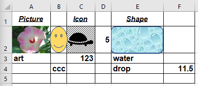
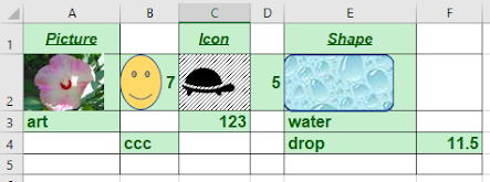
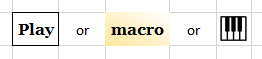
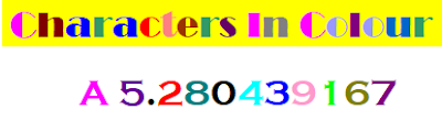
If you need to design a colorful title or banner or something similar, so that every character or group of characters or digits has a distinct color, then you can find this post helpful. Here are just two simple examples of effects you can achieve:

You can easily produce such effects quickly by entering your text (including also digits) in any cell of your worksheet, selecting the cell, and running the macro listed below. Just remember that if your cell contains just a number it must be formatted as text for this purpose.

The macro can be entered/copied into any VBA module of your workbook. Obviously, it can be modified as needed for your specific needs. Enjoy!

Sub clrFonts()
'Colors every character within a string of selected cell
Dim cnt As String
Dim rng As Range
Dim n As Long
Set rng = ActiveCell
For n = 1 To Len(rng.Value)
    cnt = Mid(rng.Value, n, 1)
    If cnt = "a" Then rng.Characters(n, 1).Font.Color = RGB(0, 0, 255): GoTo cont 'blue
    If cnt = "b" Then rng.Characters(n, 1).Font.Color = RGB(0, 255, 0): GoTo cont 'green
    If cnt = "c" Then rng.Characters(n, 1).Font.Color = RGB(255, 0, 0): GoTo cont 'red
    If cnt = "d" Then rng.Characters(n, 1).Font.Color = RGB(0, 0, 255): GoTo cont 'blue
    If cnt = "e" Then rng.Characters(n, 1).Font.Color = RGB(153, 51, 0): GoTo cont 'brownish
    If cnt = "f" Then rng.Characters(n, 1).Font.Color = RGB(255, 0, 255): GoTo cont 'd red
    If cnt = "g" Then rng.Characters(n, 1).Font.Color = RGB(0, 255, 255): GoTo cont 'green blue
    If cnt = "h" Then rng.Characters(n, 1).Font.Color = RGB(128, 0, 0): GoTo cont 'brown
    If cnt = "i" Then rng.Characters(n, 1).Font.Color = RGB(0, 128, 0): GoTo cont 'vd green
    If cnt = "j" Then rng.Characters(n, 1).Font.Color = RGB(0, 0, 128): GoTo cont 'd blue
    If cnt = "k" Then rng.Characters(n, 1).Font.Color = RGB(128, 128, 0): GoTo cont 'd grey
    If cnt = "l" Then rng.Characters(n, 1).Font.Color = RGB(128, 0, 128): GoTo cont 'vd brown
    If cnt = "m" Then rng.Characters(n, 1).Font.Color = RGB(192, 192, 192): GoTo cont 'l grey
    If cnt = "n" Then rng.Characters(n, 1).Font.Color = RGB(128, 128, 128): GoTo cont 'l green
    If cnt = "o" Then rng.Characters(n, 1).Font.Color = RGB(153, 153, 255): GoTo cont 'l blue
    If cnt = "p" Then rng.Characters(n, 1).Font.Color = RGB(153, 51, 102): GoTo cont 'vvd brown
    If cnt = "q" Then rng.Characters(n, 1).Font.Color = RGB(255, 255, 204): GoTo cont 'vl yellow
    If cnt = "r" Then rng.Characters(n, 1).Font.Color = RGB(51, 153, 102): GoTo cont 'green blue
    If cnt = "s" Then rng.Characters(n, 1).Font.Color = RGB(102, 0, 102): GoTo cont 'vvvd brown
    If cnt = "t" Then rng.Characters(n, 1).Font.Color = RGB(255, 128, 128): GoTo cont 'd orange
    If cnt = "u" Then rng.Characters(n, 1).Font.Color = RGB(0, 102, 204): GoTo cont 'vdd green
    If cnt = "v" Then rng.Characters(n, 1).Font.Color = RGB(204, 204, 255): GoTo cont 'dd grey
    If cnt = "w" Then rng.Characters(n, 1).Font.Color = RGB(0, 0, 128): GoTo cont 'vvd blue
    If cnt = "x" Then rng.Characters(n, 1).Font.Color = RGB(204, 153, 255): GoTo cont 'violet
    If cnt = "y" Then rng.Characters(n, 1).Font.Color = RGB(51, 102, 255): GoTo cont 'md blue
    If cnt = "z" Then rng.Characters(n, 1).Font.Color = RGB(102, 102, 153): GoTo cont 'greenish
    If cnt = "0" Then rng.Characters(n, 1).Font.Color = RGB(0, 0, 0): GoTo cont 'black
    If cnt = "1" Then rng.Characters(n, 1).Font.Color = RGB(0, 255, 0): GoTo cont 'green
    If cnt = "2" Then rng.Characters(n, 1).Font.Color = RGB(255, 0, 0): GoTo cont 'red
    If cnt = "3" Then rng.Characters(n, 1).Font.Color = RGB(0, 0, 255): GoTo cont 'blue
    If cnt = "4" Then rng.Characters(n, 1).Font.Color = RGB(0, 255, 255): GoTo cont 'l blue
    If cnt = "5" Then rng.Characters(n, 1).Font.Color = RGB(102, 0, 150): GoTo cont '???
    If cnt = "6" Then rng.Characters(n, 1).Font.Color = RGB(128, 128, 0): GoTo cont 'greenish
    If cnt = "7" Then rng.Characters(n, 1).Font.Color = RGB(128, 0, 128): GoTo cont 'd brown
    If cnt = "8" Then rng.Characters(n, 1).Font.Color = RGB(0, 128, 128): GoTo cont 'd green
    If cnt = "9" Then rng.Characters(n, 1).Font.Color = RGB(255, 153, 204): GoTo cont 'rouge
    If cnt Like "[A-Z]" Then
        rng.Characters(n, 1).Font.Color = RGB(255, 0, 255)  'dark red
    ElseIf cnt <> " " Then
        rng.Characters(n, 1).Font.Color = RGB(0, 0, 0)  'black
    End If
cont:
Next n
End Sub